Neural Networks explained in a mathematical way

This tutorial is synchronized with the Youtube course of Neural Networks in my youtube channel.

Nowadays, many companies take advantage of neural networks. They are used in recommendation systems, self driving cars, agriculture, smartphones and many other devices and technological sectors. But, the question is: how do they work and why are them a very important invention?

If you don’t know what a neural networks is I will explain it to you: they are computing systems inspired in biological brains but based on Calculus techniques. As our brains they have the ability to learn and decide in a intelligent way how a prototype or device must behave. Also our intelligence is enriched with different stimulus such as the sight. Artificial neural networks have also some inputs that the user must set to process and calculate the output decision or action.

For example, self driving cars have sensors that measure the distance to different obstacles. These data will be the input of the neural network. The output data will be the direction and acceleration of the car. The network will process the input data (this is what we will try to understand) and finally output how the car will move. The key, will be how we train the network and make it more intelligent. This is where we will take advantage of the calculus and in this example the network will know exactly how to process the data to avoid obstacles and follow the road.

In this post you will learn with a mathematical notation how do they perform and how do they learn internally.

Achitecture of network

Now we will start by knowing how a network is structured

We can define a neural network as a graph $G(V,A)$ where $V$ are the vertices of the graph and $A$ the arists.

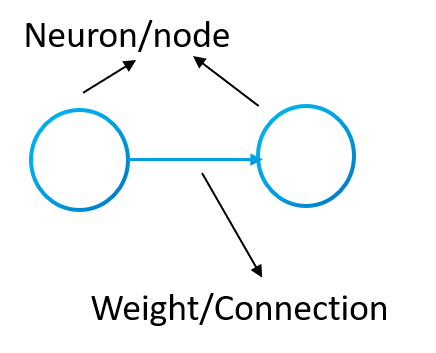
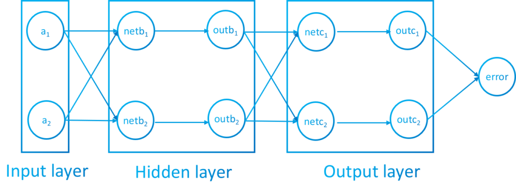
In neural networks the vertices are called neurons and the arists, connections or weights. Also each neuron will have special weights called bias. In the following image we can appreciate the neurons and weights:

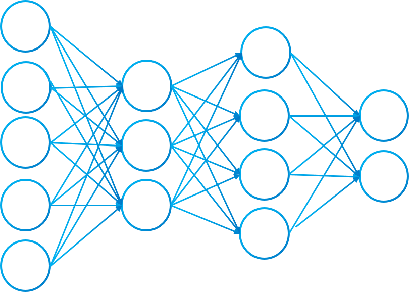
The graph of image 3 is conex and also is a digraph because every connection has a direction. Each layer is fully connected to the next (that means that every neuron of a layer is connected to every neuron of the next layer).

Also, the graph induced by two adyacent layers of neurons will be fully bipartite. If the numbers of neurons of a layer is $m$ and the number of the next layer is $n$, then we will have the bipartite subgraph $K_{m,n}$ and the number of connections between two layers will be $k=n \cdot m$

Each network will be structured in a layered architecture where each layer will contain neurons.

The topology of the neural network can be subdivided in three type of layers: INPUT LAYER, HIDDEN LAYER AND OUTPUT LAYER. The network will have only one input layer and one output layer. Each one with an specific number of neurons. However, the network can have more than one hidden layer. For instance, in picture 3 we have an input layer of 5 neurons, 2 hidden layers, one of 3 and another of 4 neurons and finally, the output layer of 2 neurons.

Every component in the network will contain values. The input layer neurons will store the data we want to analyze or use to calculate the prediction. Hidden and output neurons will calculate their values during the process of the update algorithm.

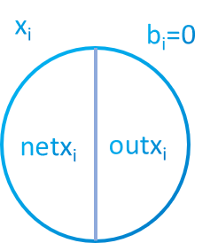
Each neuron will have two values separated by an activation function. The unactivated value will have the prefix $net$ and the value with the function applied will be $out$. To simplify notation sometimes we will be using $x_i^l$ instead of $out \ x_i^l$ where $x_i^l$ is a specific neuron in the layer $l$.

But how do we organize all the components in a mathematical structure?

In a multilayer neural network we can group neurons of a layer as a vector and the weights between 2 adyacent layers as a matrix. When we say input vector we are referring to the input neurons of the network. Same to hidden and output layer.

The vector of neurons will be denoted as $X_l$ where $l$ is the layer where the neurons are.

$$\begin{equation*}X_l=\begin{bmatrix}
x^l_1 \\\
x^l_2\\\ \vdots\\\ x^l_n
\end{bmatrix}\end{equation*}$$

We will denote an specific weight of the network as $w_{i,j}^l$ where there is a connection from neuron in position $i$ of layer $l$ to the neuron $j$ in layer $l+1$.

$$\begin{equation*}W_l=\begin{bmatrix}
w^l_{1,1} & w^l_{2,1} & \cdots& w^l_{n,1} \\\
w^l_{1,2} & w^l_{2,2} & \cdots & w^l_{n,2} \\\ \vdots & \vdots & \ddots &\vdots\\\ w^l_{1,m} & w^l_{2,m} & \cdots & w^l_{n,m}
\end{bmatrix}\end{equation*}$$

Also, we will have a vector of biases with the same size as the vector of neurons in the layer:

$$\begin{equation*}B_l=\begin{bmatrix}
b^l_1 \\\
b^l_2\\\ \vdots\\\ b^l_n
\end{bmatrix}\end{equation*}$$

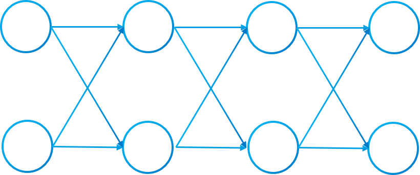
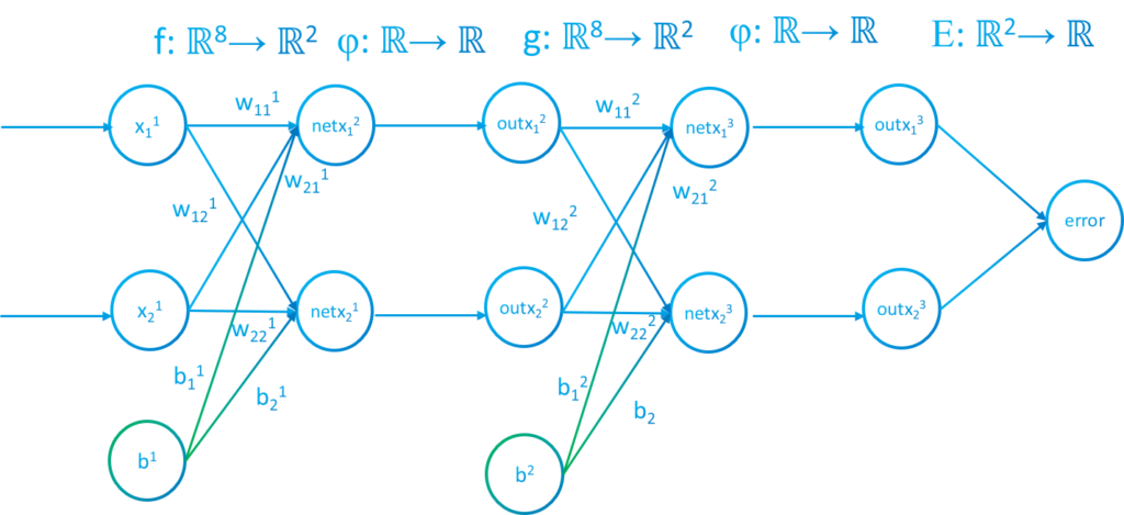
A neural network can be undestood as a composition of functions that process some inputs and outputs the error. If we analyze the image below we can see that every fully connected layer in image 1 has a function $f$ or $g$. These applications have different parameters which are neuron values, weights and biases. Also there is the activation function between each layer and finally an error function to calculate how the network is performing.

In real life problems, neural networks have more neurons and layers. For example if we want to classify digits a widely used structure is 784 input neurons (image 28×28 pixels), 2 hidden layers with 20 neurons and finally the output layer with 10 neurons (possible solutions [0,1,2,3,4,5,6,7,8,9]).

Updating the network

With all the technical parts of a network we can start to explain how the network will operate.

The process to update a neural network is known as feed-forward. With the values of the input layer vector previously setted by user we will calculate all of the values of the rest of the neurons and also the error. The input values could be pixel colors, sensor data, sound data…

In reality, each neuron will store two values that will be different. One will be calculated with the other.

As you can see in picture 4, each neuron will have to states. It will have an activation function $\phi$ that process the value of the neuron. When the neuron is not activated it will have the notation $net$, nevertheless, when the neuron is activated with the function, it will have the notation $out$. Input vector won’t be activated because its values are setted by the user.

Now we will start with the update algorithm:

Between to adyacent layers we will define an application:

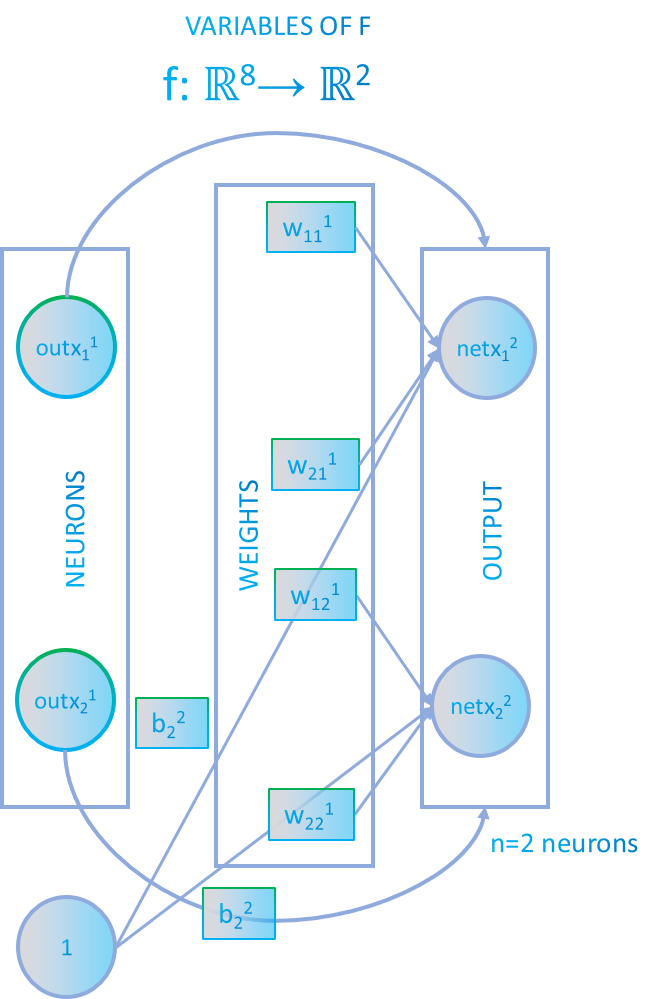
The graph induced by two adyacent layers will be a bipartite subgraph $K_{m,n}$ and it will have a linear application $f:\mathbb{R}^{(m+1)n+m}\rightarrow\mathbb{R}^{n}$. The layer function will have $m \cdot n + n + m$ variables. $m \cdot n $ to count the weights of the complete bipartite subgraph, $ n $ if we use biases and finally $m$ that are the neurons of the previous layer.

In the picture the applications of the layer are denoted as $f,g$.

Visually the function $f$ in our example will be structured as:

The vectorial function $f$ will be:

$$(net \ x_1^2 , net \ x_2^2)=\vec{f}(x_1^1,x_2^1,w_{11}^1,w_{12}^1,w_{21}^1,w_{22}^1,b_1^2,b_2^2)=(x_1^1w_{11}^1+x_2^1w_{21}^1 + b_1^2 , x_1^1w_{12}^1+x_2^1w_{22}^1+ b_2^2)$$

And $g$ will be:

$$(net \ x_1^3 , net \ x_2^3)=\vec{g}(x_1^2,x_2^2,w_{11}^2,w_{12}^2,w_{21}^2,w_{22}^2,b_1^3,b_2^3)=(x_1^2w_{11}^2+x_2^2w_{21}^2 + b_1^3 , x_1^2w_{12}^2+x_2^2w_{22}^2+ b_2^3)$$

We can appreciate that they are continuous in $\mathbb{R}^{(m+1)n+m}$ because it´s a linear function. The function is also diferentiable because the class is $C^{\infty}$

General formula

We have layer $L_1$ with the neurons ${x_1,^l,x_2^l,…,x_m^l}$ and $L_2$ with neurons ${x_1^{l+1},x_2^{l+1},…,x_n^{l+1}}$. Weights will have the notation $w_{i,j}^l$ when it connects $x_i^l$ and $x_j^{l+1}$. Biases will have the form $b_j^l$ associated to the neuron $x_j^l$ . To simpify notation $x_i^l = out \ x_i^l$ .Then, the update process of the network will be:

$$net \ x_j^{l+1}=\sum_{i=1}^{m}{x_i^lw_{ij}^l}+b_j^{l+1}$$

$$out \ x_j^{l+1}=\phi(net \ x_j^{l+1})$$

We can update a layer using the matrix form of a linear application. Layer $l+1$ has $m$ neurons and layer $l$, $n$ neurons:

$$net \ X_{l+1}=W_l \cdot out \ X_l+B_{l+1}=\begin{bmatrix}
net \ x^{l+1}_1 \\\
net \ x^{l+1}_2\\\ \vdots\\\ net \ x^{l+1}_m
\end{bmatrix}=\begin{bmatrix}
w^l_{1,1} & w^l_{2,1} & \cdots& w^l_{n,1} \\\
w^l_{1,2} & w^l_{2,2} & \cdots & w^l_{n,2} \\\ \vdots & \vdots & \ddots &\vdots\\\ w^l_{1,m} & w^l_{2,m} & \cdots & w^l_{n,m}
\end{bmatrix}\begin{bmatrix}
out \ x^l_1 \\\
out \ x^l_2\\\ \vdots\\\ out \ x^l_n
\end{bmatrix}+\begin{bmatrix}
b^{l+1}_1 \\\
b^{l+1}_2\\\ \vdots\\\ b^{l+1}_m
\end{bmatrix}$$

$$out\ X_{l+1}=\phi (net \ X_l)=\begin{bmatrix}
out \ x^{l+1}_1 \\\
out \ x^{l+1}_2\\\ \vdots\\\ out \ x^{l+1}_m
\end{bmatrix}=\phi \left(\begin{bmatrix}
net \ x^{l}_1 \\\
net \ x^{l}_2\\\ \vdots\\\ net \ x^{l}_m
\end{bmatrix}\right)$$

Each layer will be updated with the previous layer output. When the network execute the $f$ function it will obtain $x_1^2$ and $x_2^2$ values so we will be able to execute $g$ with that values previously obtained.

These applications are diferenciable because they are of class $C^{\infty}$ and also their are linear applications. Therefore, we can use the powerful tools of diferentiable Calculus.

The logistic function is widely used for learning curves so in this example we will be using it. For more activation functions see: Activation functions

$$\phi(x)=\frac{1}{1+e^{-x}}$$

Example of the update process

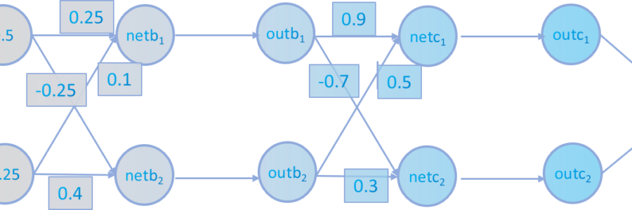
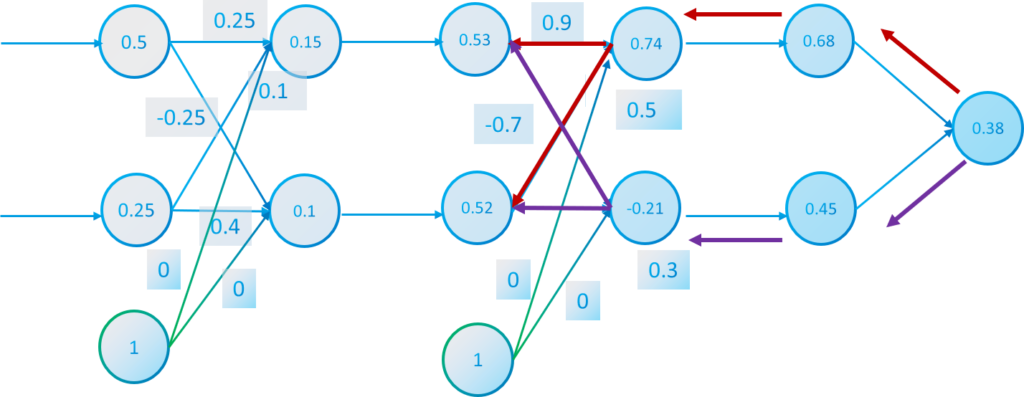
First of all we have the weights setted, the input layer values which are 0.5 and 0.25 and the bias is 0 at the initial state.

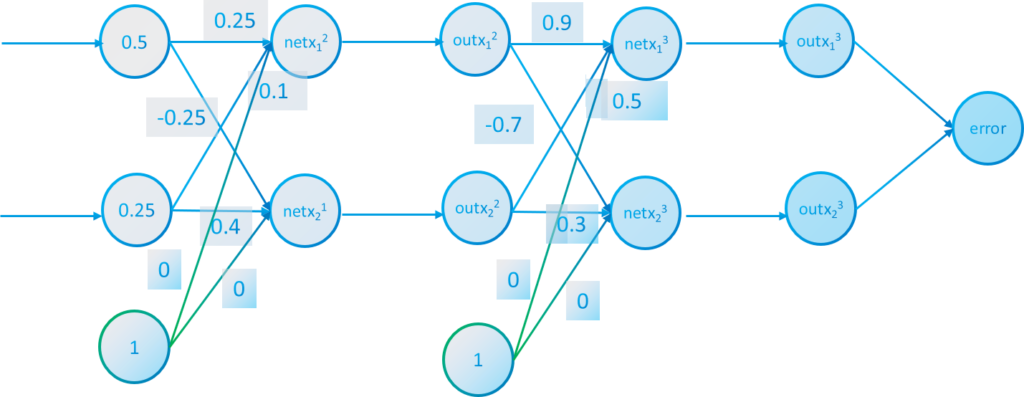
We execute the update process of the first layer with the formula. The red arrows apply the feedforward process activation function.

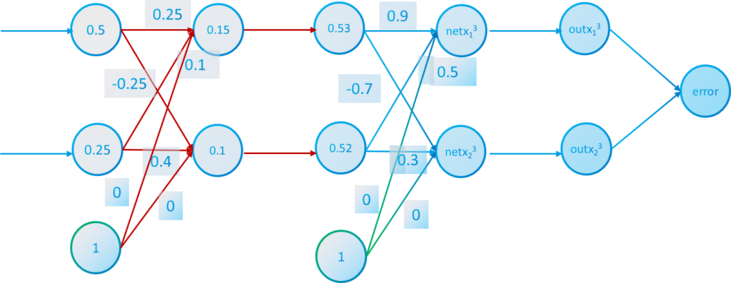
$$net \ x_1^2= 0.5 \cdot 0.25 + 0.25 \cdot 0.1 + 0 = 0.15 \quad out \ x_1^2=\frac{1}{1+e^{-0.15}}=0.53$$

$$net \ x_2^2= 0.5 \cdot 0.35 + 0.25 \cdot (-0.3) + 0 = 0.1 \quad out \ x_2^2=\frac{1}{1+e^{-0.1}}=0.52$$

Then with the values of $out \ x_1^2 $ and $out \ x_2^2$ we can do a step forward and calculate the values of $x_1^3$ and $x_2^3$

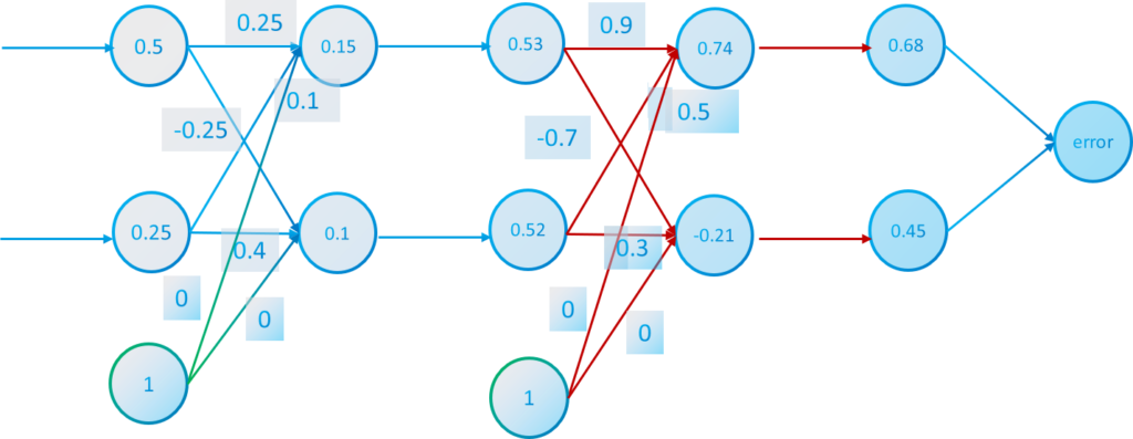
$$net \ x_1^3= 0.53 \cdot 0.9 + 0.52 \cdot 0.5 + 0 = 0.74 \quad out \ x_1^3=\frac{1}{1+e^{-0.74}}=0.68$$

$$net \ x_2^3= 0.53 \cdot (-0.7) + 0.52 \cdot 0.3 + 0 = -0.21 \quad out \ x_2^3=\frac{1}{1+e^{0.21}}=0.45$$

With the feed-forward process we have calculated every value of every neuron. Now we need to calculate the error that the network has done to learn.

Calculating the error

If we have datasets to train, we can calculate the error the network has done to an specific data point. Imagine that the dataset contains different data each one with the input values we want to give the network and also the output solution the network should return.

For example the input data in our example network is $[x_1^1=0.5, x_2^2=0.25]$ and the desired output data we cant the network to return is $[d_1=0, d_2=1]$. Clearly, the output solution of the network hasn’t been accurate $[x_1^3=0.68, x_2^3=0.45]$.

We want to measure the error the network have had. A technique the networks have is to implement a cost function that measures the difference between two vectors (desired and real output) . In this case we will be using the Mean Squared Error (MSE):

With the desired values we will calculate the differences between the real value and the desired.

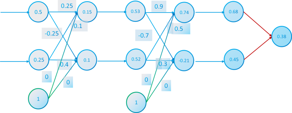
$$E(x_1^3,x_2^3)=\frac{(d_1-x_1^3)^2+(d_2-x_2^3)^2}{2}=\frac{(-0.68)^2+(0.55)^2}{2}=0.38$$

The general form of the error is where $x_j$ is the neuron in position $j$ of the output layer neurons and $d_j$ the desired value in that position.

$$E(\vec{x})=\frac{\sum_{j=1}^{n}{(d_j-x_j^L)^2}}{n}$$

The size of the output layer is $n$.

If we want it in a matrix form denoting the output vector as $X$. Also, $Y$ will be the desired vector and $n_L$ the number of neurons in output layer:

$$E(X_L)=\frac{1}{n_L}(Y-X_L) \cdot (Y-X_L)^t$$

Training the network

The previous network was randomly chosed. But what if we want to calculate the weights to fit to a problem a not chosen them randomly?. In other words, why if we adjust every weight and bias in the network to decrease the error. This is the general idea of the training process of a neural network. We want to update every weight and bias to improve the performance of the network. This is not easy and requires Calculus to solve this problem.

When the network is created we must initialize randomly the weights to start at a point. A good way to initialize the weights is with a normal distribution function between [-1,1]. Biases are usually initialize with a zero value but the can also be intialized randomly

The problem comes when we want to optimize the weights and biases to reduce the error. These elements are a type of regulators the network must adjust to decrease the cost function..

We can think of an optimization problem where we want to minimize the error. However, is important to don’t overfit the neural network. In other terms, we dont want to decrease the error a lot because in an iteration we are learning with a certain data but the network must learn about the entire dataset. There are a lot of waysto prevent overfitting. One of them is to have a learning rate.

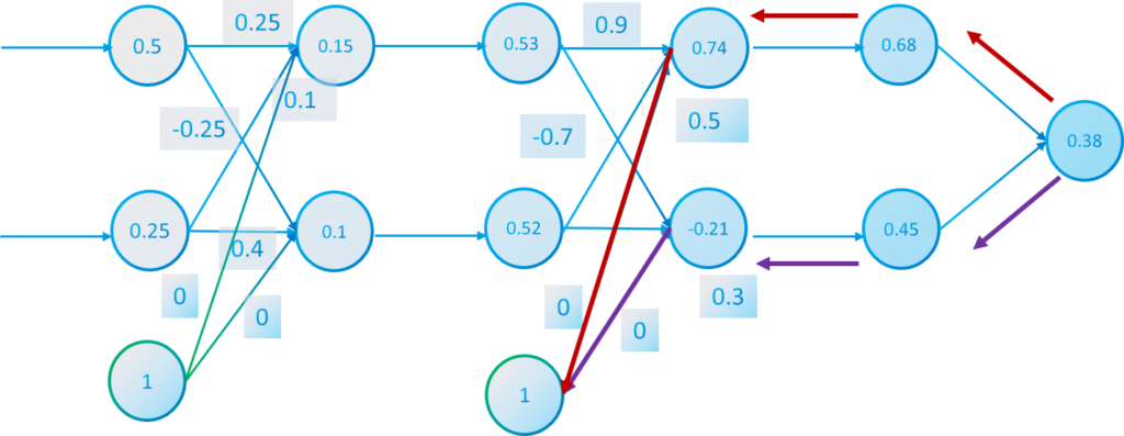
But in a mathematical way how do we adjust every weight to reduce the error. Thanks to diferentiable Calculus it’s possible. In neural network the process to adjust every weight is known as back-propagation and it will process the network in the opposite direction as the feed-forward

Gradient descent is a great tool to reduce error in a multidimensional space and with composition of functions. We are questioning about:

$$\frac{\partial E(\vec{x})}{\partial w^l_{ij}}$$

Applying the chain rule we can calculate every weight in the network. In the example network we have 8 weights to adjust.

Calculating adjustments of last layer weights and biases

The way we calculate the derivatives between one layer and another will be different because of the chain rule. First layers in network will have more operations to calculate their derivatives

$$\frac{\partial E(\vec{x})}{\partial w^{L-1}_{ij}}=\frac{\partial E}{\partial out \ x^{L}_{j}}\frac{\partial out \ x^L_{j}}{\partial net \ x^L_{j}} \frac{\partial net \ x^L_{j}}{\partial w^{L-1}_{ij}}$$

If we calculate the derivatives knowing that we are using the logistic function and MSE error:

$$\frac{\partial E(\vec{x})}{\partial w^{L-1}_{ij}}=\frac{-2(d_j-x_j^L)}{n}\phi ‘ (net \ x_j^L) out\ x_i^{L-1}$$

The first term is the derivative of the MSE error and the last term the derivative of the feed-forward function. Now, if $\phi$ is the logistic function then:

$$\phi ‘ (net \ x_i^l)=\phi(net \ x_i^l)(1-\phi(net \ x_i^l))=out\ x_i^l(1-out\ x_i^l)$$

We can define a term that is the error signal $\delta _i^l$ that will be stored in each neuron and will accumulate the chain rule derivatives in that specific layer. These will help to calculate the derivatives in the other layers.

$$\delta_j^l=\frac{\partial E}{\partial net\ x^{l}_{j}}=\frac{\partial E}{\partial out \ x^{l}_{j}}\frac{\partial out \ x^l_{j}}{\partial net \ x^l_{j}}$$

So the formula to calculate the weights will be:

$$\frac{\partial E(\vec{x})}{\partial w^{L-1}_{ij}}=\delta_j^L \frac{\partial net \ x^L_{j}}{\partial w^{L-1}_{ij}}$$

For example if we calculate every partial derivative of a weight of $W_2$ with respect to $E$ will be:

$$\frac{\partial E(x_1^3,x_2^3)}{\partial w_{11}^2}=\frac{-2(0-0.68)}{2}(0.68)(1-0.68)0.53=0.078$$

$$\frac{\partial E(x_1^3,x_2^3)}{\partial w_{21}^2}=\frac{-2(0-0.68)}{2}(0.68)(1-0.68)0.52=0.077$$

$$\frac{\partial E(x_1^3,x_2^3)}{\partial w_{12}^2}=\frac{-2(1-0.45)}{2}(0.45)(1-0.45)0.53=-0.07$$

$$\frac{\partial E(x_1^3,x_2^3)}{\partial w_{22}^2}=\frac{-2(1-0.45)}{2}(0.45)(1-0.45)0.52=-0.07$$

We can also represent all the derivatives in the Jordan matrix $J$:

$$\frac{\partial E}{\partial W_{L-1}}=\begin{bmatrix}
\frac{\partial E}{\partial w^{L-1}_{1,1}} & \frac{\partial E}{\partial w^{L-1}_{2,1}} & \cdots& \frac{\partial E}{\partial w^{L-1}_{n,1}}\\\
\frac{\partial E}{\partial w^{L-1}_{1,2}} &\frac{\partial E}{\partial w^{L-1}_{2,2}} & \cdots & \frac{\partial E}{\partial w^{L-1}_{n,2}} \\\ \vdots & \vdots & \ddots &\vdots\\\ \frac{\partial E}{\partial w^{L-1}_{1,m}}& \frac{\partial E}{\partial w^{L-1}_{2,m}} & \cdots &\frac{\partial E}{\partial w^{L-1}_{n,m}}
\end{bmatrix}=\left(\begin{bmatrix}
\frac{\partial E}{\partial out \ x^{L}_{1}} \\\
\frac{\partial E}{\partial out \ x^{L}_{2}}\\\ \vdots\\\ \frac{\partial E}{\partial out \ x^{L}_{n}}
\end{bmatrix}\odot\begin{bmatrix}
\frac{\partial out \ x^{L}_{1}}{\partial net \ x^{L}_{1}} \\\
\frac{\partial out \ x^{L}_{2}}{\partial net \ x^{L}_{2}}\\\ \vdots\\\ \frac{\partial out \ x^{L}_{n}}{\partial net \ x^{L}_{n}}
\end{bmatrix}\right)\begin{pmatrix}
\frac{\partial net \ x^{L-1}_{1}}{\partial w^{L-1}_{.j}}&
\frac{\partial net \ x^{L-1}_{2}}{\partial w^{L-1}_{.j}}& \cdots&& \frac{\partial net \ x^{L-1}_{m}}{\partial w^{L-1}_{.j}}
\end{pmatrix}$$

If we want to express it with the error signal $\delta$ :

$$\frac{\partial E}{\partial W_{L-1}}=\delta _{L} \cdot (X_{L-1})^T=\left(\begin{bmatrix}\frac{-2(d_1-x_1^L)}{n} \\\frac{-2(d_2-x_2^L)}{n}\\ \vdots \\ \frac{-2(d_n-x_n^L)}{n}\end{bmatrix}\odot\begin{bmatrix}\phi'(net \ x_1^{L}) \\ \phi'(net \ x_2^{L})\\ \vdots \\ \phi'(net \ x_n^L)\end{bmatrix}\right)\begin{pmatrix}out \ x_1^{L-1}&out \ x_2^{L-1}&\cdots&out \ x_n^{L-1}\end{pmatrix}$$

Now we will learn how to calculate the derivatives with respect to each bias:

$$\frac{\partial E}{\partial b^L_{j}}=\frac{\partial E}{\partial out \ x^L_{j}}\frac{\partial out \ x^L_{j}}{\partial net \ x^L_{j}}\frac{\partial net \ x^L_{j}}{\partial b^L_{j}}$$

The last derivative if one because the bias neuron has always a value of 1.

$$\frac{\partial E}{\partial b^L_{j}}=\frac{\partial E}{\partial out \ x^L_{j}}\frac{\partial out \ x^L_{j}}{\partial net \ x^L_{j}}\cdot 1=\delta _j^L $$

Then the derivatives will be:

$$\frac{\partial E}{\partial b^L_{j}}=\frac{-2(d_j-x_j^L)}{n}\phi ‘ (net \ x_j^L) $$

In a matrix form

$$\frac{\partial E}{\partial B_{L}}=\begin{bmatrix}
\frac{\partial E}{\partial b^L_1} \\\
\frac{\partial E}{\partial b^L_2}\\\ \vdots\\\ \frac{\partial E}{\partial b^L_n}
\end{bmatrix}=
\delta _L=\left(\begin{bmatrix}
\frac{\partial E}{\partial out \ x^{L}_{1}} \\\
\frac{\partial E}{\partial out \ x^{L}_{2}}\\\ \vdots\\\ \frac{\partial E}{\partial out \ x^{L}_{n}}
\end{bmatrix}\odot\begin{bmatrix}
\frac{\partial out \ x^{L}_{1}}{\partial net \ x^{L}_{1}} \\\
\frac{\partial out \ x^{L}_{2}}{\partial net \ x^{L}_{2}}\\\ \vdots\\\ \frac{\partial out \ x^{L}_{n}}{\partial net \ x^{L}_{n}}
\end{bmatrix}\right)$$

Let’s continue with the example

$$\frac{\partial E(x_1^3,x_2^3)}{\partial b_1^3}=\frac{-2(0-0.68)}{2}(0.68)(1-0.68)=0.15$$

$$\frac{\partial E(x_1^3,x_2^3)}{\partial b_2^3}=\frac{-2(0-0.45)}{2}(0.45)(1-0.45)=-0.13$$

Calculating adjustments of the rest of weights and biases

In the rest of the layers to calculate the derivatives of the weights and biases we will continue applying the chain rule. However to optimize the network we will be using the derivatives previous calculated.

$$\frac{\partial E}{\partial out \ x^l_j}=\sum_{i=1}^n{\frac{\partial net \ x_i^{l+1}}{\partial out \ x^l_j}\frac{\partial E}{\partial net \ x^l_j}}=\sum w_{ji}^l \delta _j^l$$

We will use the error signal as $\delta$ which will be associated to every neuron in a layer and it will store its derivative

$$\delta _j^l=\frac{\partial E}{\partial net \ x^l_{j}}=\frac{\partial E}{\partial out \ x^l_{j}}\frac{\partial out \ x^l_{j}}{\partial net \ x^l_{j}}=\left(\sum {w_{ji}^l \delta _j^{l+1}}\right) \phi´(net x_j^l)$$

So now we can calculate the derivative with respect to every weight:

$$\frac{\partial E}{\partial w_{ij}^l}=\frac{\partial E}{\partial net \ x^l_{j}}\frac{\partial net \ x^l_{j}}{\partial w_{ij}^l}=\delta _j^l x_i^{l-1}$$

Updating weights and biases

With all the derivatives calculated we can now update the weights and biases. We want to decrease the error (minimize). $\eta$ will be the learning rate previosly mentionated.

$$w_{ij}^l=w_{ij}^l-\eta\frac{\partial E(\vec{x})}{\partial w^l_{ij}}$$

The negative sign is because we want to decrease the error.

Another way to understand the optimization is with the gradient vector.

$$w_{.j}^l=w_{.j}^l-\eta\nabla(f_i)$$

If we update the biases:

$$b_{j}^l=b_{j}^l-\eta\frac{\partial E(\vec{x})}{\partial b^l_{j}}$$

If we use matrixs:

$$W_l=W_l-\eta J(\vec{f})=\begin{bmatrix}
w^l_{1,1} & w^l_{2,1} & \cdots& w^l_{n,1} \\\
w^l_{1,2} & w^l_{2,2} & \cdots & w^l_{n,2} \\\ \vdots & \vdots & \ddots &\vdots\\\ w^l_{1,m} & w^l_{2,m} & \cdots & w^l_{n,m}
\end{bmatrix}-\eta\begin{bmatrix}
\frac{\partial E}{\partial w^l_{1,1}} & \frac{\partial E}{\partial w^l_{2,1}} & \cdots& \frac{\partial E}{\partial w^l_{n,1}}\\\
\frac{\partial E}{\partial w^l_{1,2}} &\frac{\partial E}{\partial w^l_{2,2}} & \cdots & \frac{\partial E}{\partial w^l_{n,2}} \\\ \vdots & \vdots & \ddots &\vdots\\\ \frac{\partial E}{\partial w^l_{1,m}}& \frac{\partial E}{\partial w^l_{2,m}} & \cdots &\frac{\partial E}{\partial w^l_{n,m}}
\end{bmatrix}$$

$$B_l=B_l-\eta (\nabla(\phi _l)^t)=\begin{bmatrix}
b^l_1 \\\
b^l_2\\\ \vdots\\\ b^l_n
\end{bmatrix}-\eta \begin{bmatrix}
\frac{\partial E}{\partial b^l_{1}} \\\
\frac{\partial E}{\partial b^l_{2}}\\\ \vdots\\\ \frac{\partial E}{\partial b^l_{n}}
\end{bmatrix}$$

Training and test process

With the feed-forward and back-propagation techniques the network can learn a certain dataset and return accurate results.

We can update the parameter of the network in different moments. The default way is to adjust them on each data element iteration. This is called Stochastic Gradient Descent (SGD). However it has been proved that if we specify a minibatch size (32,64,128,…) and adjust the parameters when the minibatch has been iterated it will have a better performance in the optimization of the network training process.

The training process will have some step the network should do

Requisites for training and testing

• Create architecture of network

The network layers, parameters and topology must be set

• Initialize

The network should initialize all parameters including the weights and biases. We can use for the weights a random initialization between [-k,k] (k is recommended to be 1) or a normal random distribution. The bias are usually set to zero.

• Load dataset

We need to load the dataset and store it in RAM. However if the dataset is to large we can split it in different batches to reduce the memory used.

Training process

We need to calculate the minibatch size depending on the size of minibatch we want to use and the dataset size.

• For each epoch
  • Shuffle data of dataset (randomize the position of the data)
  • For each minibatch
    • For each iteration in minibatch:
      • Assign the inputs of dataset in that iteration position to the input layer
      • Apply the feed-forward function to calculate outputs
      • Calculate error (optional)
      • Back-Propagation using the desired output in the dataset in that iteration position. This will calculate the derivatives of each weight and bias
    • Adjust with the gradient descent technique each weight and bias (weights and biases derivatives will be accumulated in a matrix for each iteration) and finally divided by the minibatch size.
    • Reset gradient matrixs (set to zero)

Optional: we can also graph the error to see the performance in a 2D graph.

Test process

In this case we will have another dataset different from the training dataset to test the network.

• For each iteration in dataset:
  • Assign the inputs of dataset in that iteration position to the input layer
  • Apply the feed-forward function to calculate outputs
  • Calculate error with outputs and desired values of dataset
  • Accumulate error (optional)

• Stadistics
  • Output the mean error dividing the accumulate error by the dataset size

Using the network

When the network has been trained successfully with a low error. We can start to take advantage of it and without using desired outputs values. In this moment we don´t know the output and we want the network to predict it.

To give a prediction of the network:

• Assign the inputs to analyze to the input layer
• Apply the feed-forward function to calculate outputs

With this post you will know how a neural network work internally and the maths behind it. You will now be able to use AI libraries and apply the feed-forward neural network or implement your own neural network from scratch.

I hope this post have helped to you. In that case you can give feedback.