Optimization Algorithms in Neural Networks

Neural Networks are complex models that can be trained to get better results and predictions. This training sometimes is fast and useful but others not. This is because the Gradient Descent algorithm of back-propagation is not always the best. This can be solved with optimization algorithms that improve the accuracy of the model and also the speed.

When we train the network we can now if the gradient descent is working well or not analyzing the error.

Calculating the Error

The error is very important to analyze the performance of our neural model. We have two main formulas to calculate the error.

The error will be calculated with the sum of the output neuron values in different ways:

• Mean Squared Error (MSE)

$$E(x)=\frac{1}{2}\sum_o{(x-d)^2}$$

Where $x$ is the obtained value and $d$ the desired value.

The square pow is only used to have only positive values. We can also you the absolute valor of the difference:

$$E(x)=\frac{1}{2}\sum_o{\mid x-d\mid}$$

• Cross Entropy

$$E(x)=\sum_o{d\log{x}}$$

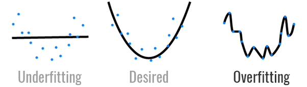
Also depending on the learning we apply to the model, we will have three posibilities:

• UNDERFITTING: the model is not accurate and is very flexible. When we train with a dataset, the error is always high. This happens when the learning rate of the network is very low.
• OVERFITTING: this situation comes up when we try in a very accurate way. We learn with a high learning rate almost 1 so we will decrease the full gradient in one training set
• DESIRED: the best way to learn is the middle term between the two situations explained before. We want to be flexible with the training sets to learn from everyone but also to try to decrease the error remarkably.

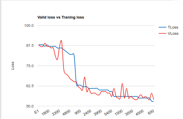
Also we can understand the behavior of the network with the error function during the epochs. When we are training we will have a function that decreases (training loss). In the test of the neural network (valid loss) we will have another function. If they are very similar like the example here the network will have a good performance.

The fluctuations of the error usually mean a good factor of the performance of the network. Also the error should decrease during the time passed (epochs)

To get very similar result of the two functions valid loss and training loss we can use different optimization algorithms:

• Gradient Descent Variants
• Gradient Descent Optimization Algorithms

The first type were explained in the Feed-Forward Neural Network Tutorial where the mini-batch, batch and stochastic gradient descents were analyzed.

Gradient Descent Optimization Algorithms

We have a great variety of optimization algorithms. Some of them increase the speed of approach to the minimum, other have a dynamic learning rate to reach the best minimum and other have both of them.

In this animation you can watch the different optimization algorithms and which ones reach the best minimum and the epochs it take to each one.

The gradient descent value calculated in the back-propagation will be $g_t$ that will be equivalent to all of the $\frac{\partial E}{\partial w}$ where $E$ is the error. $\theta$ will be the matrix with all the weights.

Momentum

This optimization algorithm helps to accelerate the Stochastic Gradient Descent in the relevant direction, reducing the oscillations in the wrong directions and stimulating the direction to the minimum.

$$v_t=\lambda v_{t-1}+\mu g_t$$

Finally to update each weights:

$$\theta =\theta – v_t$$

The momentum term $\lambda$ will be 0.9 or a similar value.

Nesterov Gradient Descent (NAG)

With the momentum the descent is following the slope blindly. We want to use smarter movements so when the error is approaching to the minimum the speed will decrease.

$$v_t=\lambda v_{t-1}+\mu g_t(\theta-\lambda v_{t-1})$$