Feed-Forward Neural Network

A Feed-Forward Neural Network was the first model that was invented and implemented for machine learning. Its inspired in the biological brains and they are widely used because they can learn an specific task. With some input data, the neural network will generate some output that will be the predictions.

However, if we want to have good predicted values we should train the neural network with lot of examples. When we finished the training the neural network will be able to give accurate results as outputs.

As we saw in the last post of Neural Networks we have different ways to learn and train the neural network. Depending on the problem we want to face we will use an specific way of learning. For image classification, supervised learning is a good idea. In this tutorial we use the learning algorithm.

Neural Network Architecture

The architecture of a feed forward neural network consists on some layers that contain neurons. This neurons are fully connected to the neurons of the next and previous layer.

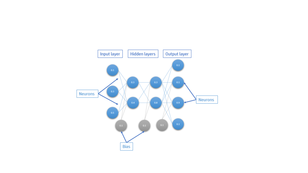
Each neurons, weight and bias store a value. Depending on the position of the layer it will have a different name:

• Input layer: all the data we want to predict is stored on this input neurons
• Hidden layers: contain the neurons that are between the output and input layer. It improves the intelligent of the neural network
• Output layer: predicted values of the network.

Training Steps

For having a better neural network that gives accurate results we will need to train it. Because we are using supervised learning we will use the back-propagation algorithm. We will have labelled data so we will have the input values of the data and also the outputs it must give. With this outputs we will be able to calculate the error. The reduction of the error will be done with the gradient descent algorithm where we will try to go to the best local minimum error. This could be improved with optimization algorithms.

To train the model will be divided in:

1. Initialization: all the weights will be randomly filled with values in the range [-1,1]
2. Training loop: iterate through all the dataset
   • Feed-Forward: updating
   • Calculate error
   • Back-Propagation: training
   • Update weights and biases

Feed-Forward

Moreover, to update the network we will use the Feed-forward function. With some inputs in the input layer, the weights and the bias we will update the neurons of the hidden layers and the output layers.

\[o_m^{l+1}=\sigma(\sum{w_{m,n}^{l} \cdot o_n^l+b^l}) \]

We will start in the first layer and we will and go forward in the neural network. $m$ is the position of the neuron we want to calculate the value, $o$ is a neuron, $w$ is a weight that connects $m$ and $n$ neuron positions. $b$ is the bias in the layer position $l$.

When we finally sum up all the values we will get the $net$ value of the neuron if we want to get the final value $out$ we will need to apply the activation function $\sigma(net)$

Depending on the activation we want to do we will have:

Linear

\[ out = net$ \]

RELU

\[ out=\begin{cases} net, & net>0 \\ 0, & net<0 \end{cases} \]

Sigmoid

\[ out=\frac{1}{1+e^{-net}} \]

Hyperbolic tanh

\[ out=\frac{e^{net}-e^{-net}}{e^{net}+e^{-net}} \]

With this we will be updating the entire network.

Calculate error

The error should be calculated each iteration of the training loop:

\[ E = \frac{1}{2}\sum{(out_m^l-d_m^l)^2} \]

Where $l$ is the last layer output predictions, $d$ is the desired value (labelled data) and $out_m$ the outputs prediction of the network that must be improved.

Back-Propagation

To train the model we will need to reduce the error.

We will calculate the partial derivative of the error with repect to each weight. Applying the chain rule we will get:

\[\dfrac{\partial E_{total}}{\partial w_{m,n}}=\dfrac{\partial E_{total}}{\partial out(a_n^l)}\dfrac{\partial out(a_n^l)}{\partial{ net(a_n^l)}}\dfrac{\partial net(a_n^l)}{\partial w_{m,n}}\]

Output layer back-propagation

Solving the partial derivatives where $a_n^l$ is the $out$ activation, $\sigma’$ is the derivative of the activation function

The derivative of the error is:

$$\dfrac{\partial E_{total}}{\partial out(a_n^l)} = -(x_{n}^l-a_{n}^l) $$

Doing every derivative we have:

$$\dfrac{\partial E_{total}}{\partial w_{m,n}}=-(x_{n}^l-a_{n}^l) \sigma'(a_n^l)a^{l-1}_m=\delta_n^l a_m^{l-1} $$

If the activation is the sigmoid function its derivative will be:
$$\sigma'(x)=\sigma(x)(1-\sigma(x))$$

We should then create a new important term called error signal that will be the error we will propagate through the neural network in the opposite direction of the feed-forward (from the outputs to the inputs). It won’t depend on the previous neuron of the weight we want to calculate the error.

$$\delta_n^l=-(x_{n}^l-a_{n}^l) \sigma'(a_n^l)$$

Hidden layer back-propagation

Each new derivative now will depend on the previous neurons so the calculations will change.

$$\delta_n^{l+1}=\sum_{m=0}(\delta_m^l w_{m,n}^{l+1}) $$

Finally we will have:

$$\dfrac{\partial E_{total}}{\partial w_{m,n}}=\left(\sum_{m=0}(\delta_m^l w_{m,n}^{l+1})\right)\sigma’a^{l-1}_n$$

If we want to calculate the error with respect to each bias it won’t depend on the previous neuron value because it will be one so we will have the next formula:

$$\dfrac{\partial E_{total}}{\partial b_{m}^l}=\delta_m^l$$

General Formula

With all of this calculations we can conclude that we can obtain the variaton of each weight to decrease the error with the following formula:

$$\dfrac{\partial E_{total}}{\partial w_{m,n}}= \delta_n^l a_m^{l-1} $$

And for the bias:

$$\dfrac{\partial E_{total}}{\partial b_{n}}= \delta_n^l $$

Where the $\delta$ will be calculated different depending on the layer.

All the calculations and ideas are shown in the next video:

Updating the weights and biases

When we have every derivative calculated for every weight and bias we will need to use it for decreasing the error of the neural network.

We will define $\mu$ as the learning rate of the network. This learning rate is constant but with some optimization algorithms we will be able to change it during the train.

There are different ways to update all the weights and biases.

• Stochastic Gradient Descent

It’s the normal way of updating the network. We update each all the network weights and biases on each training. It’s the fastest way and the less memory it takes but it’s not the most efficient way to update the network.

$$w_{m,n}^l= w_{m,n}^l-\eta\dfrac{\partial E_{total}}{\partial w_{m,n}} $$

• Batch Gradient Descent

It’s takes much memory because it updates the network when all the training sets derivatives have been calculated. It can also produce overfitting of the network. It’s not recommendable.

• Mini-Batch Gradient Descent

It’s a middle term between the other optimization gradient descents. It update all the elements of the network in a mini-batch of normally between 64-256 training data. It doens’t consume a lot of memory and it approaches fast to the minimum.

$$w_{m,n}^l= w_{m,n}^l-\eta\dfrac{1}{s}\sum_{s=0}^{s}\dfrac{\partial E_{total}}{\partial w_{m,n}} $$

Gradient descent algorithms are explained in the next video:

If you have any question you can add a comment here.