Convolutional Neural Networks

Convolutional Neural Networks are widely used for image classification. With some filters we can simplify an colored image with its most important parts. The main feature of a Convolutional Network is the convolution operation where each filters goes over the entire input image and creates another image.

Also you can watch the video where I explain how they work in a simple way. The Convolutional Neural Network tutorials also will explain the code to create it and represent it in a 3D visualization.

A ConvNet or Convolutional Neural Network (CNN) is a complex model of artificial intelligence that outputs some prediction of certain inputs. It includes a Feed-Forward Neural Network layer but also some special layers we will analyze soon.

They are used for important companies such as Google, Nvidia for image classification, autonomous cars, speech recognition, face detection and camera. The convolution operation is an operator that can easily create different image effects with some filters that change the aspect of the image. In Artificial Intelligence is often used for edge detection.

Convolutional Neural Network

Convolutional Neural Networks are mainly used to analyze RGB images. These images will perform as the input data of the neural network. RGB images often require more performance to be analyzed. There are many more weights to process than in the traditional multilayer Feed-Forward Neural Network. It will have a higher computational cost. With ConvNets, we can simplify the image and get the most important parts of it to decrease the input data that will be processed afterwards.

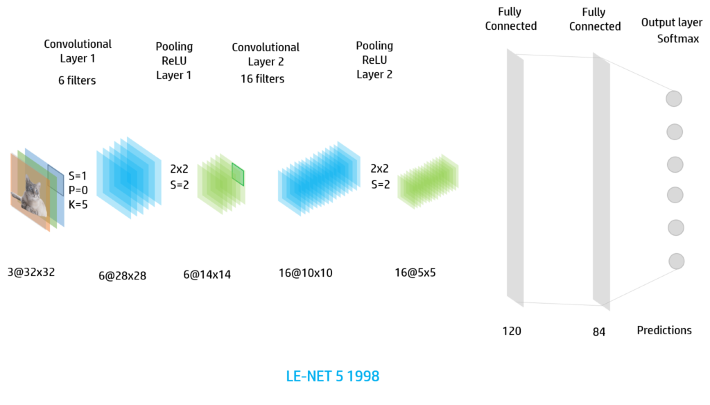
This networks will have different layer depending on their functionalities and features:

• Convolutional Layer
• Activation Layer
• Pooling Layer
• Fully connected Layer
• Output Layer

Some of this layers will be repeated in a ConvNet architecture more than one time.

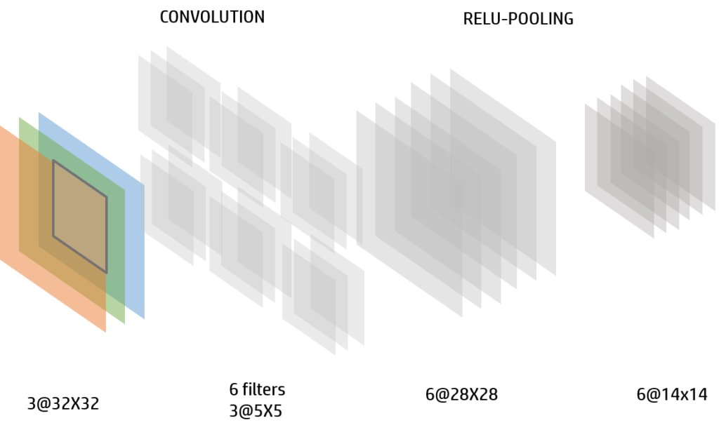
In the image we have the most typical layers of the Convolutional Neural Network. The input data is an image RGB and will proccess it with the different layers.

The activation layer, fully connected layer and output layer are very similar to the Feed-Forward Neural Network. However they have also some differences.

FEATURE IMAGES

To undestand deeply how these neural networks work, we will need to define some terms:

Each image that is created with the convolution operation, pooling or activation function and the input image will be a feature image. This images will have some size. They will have a normal width (W)and height (H) but also depth or number of channels (C) of the image.

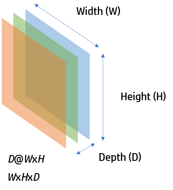
In the input RGB image will have 3 channels: red, green and blue. This size will be represented with the next notation D@WxH

We will start with those of the Convolutional Neural Network.

CONVOLUTIONAL LAYER

This is the most important layer. It’s defined as an special operation that we will apply to a channel with a filter. This filter (F) will have weights and a bias that will be the parameters with which the neural network will learn.

These filters or also named kernels that will be used to create the output image of the layer. They will have to be the same depth as the input image. However the size k x k of the kernels will need to be less than the size of the feature image.

We can apply as many filters as we want. In the next example there are 6 filters. The output image will have the depth of the amount of filters we have, in this case 6.

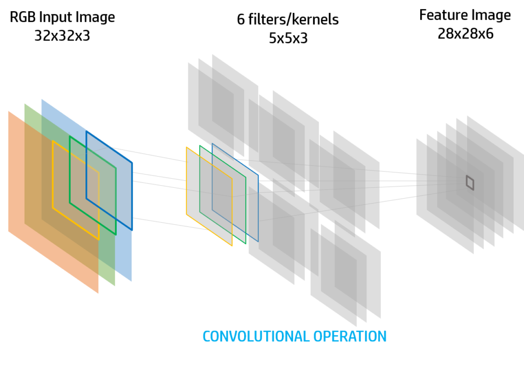
Convolutional operation is similar to the cross-correlation but the kernel will be “flipped”. The input image will be denoted with I and the output image C.

So the convolutional operation will be will be the equivalent in to the feed-forward function of a multilayer neural network:

$$C(x,y)=I * F=\sum_{m=0}^{k-1}{\sum
_{n=0}^{k-1} {\sum_{C}{K_{m,n,c}\cdot I_{i+m,j+n,c}+b}}} $$

The filter values will be firstly initialized with a normal distribution or complete random in the range [-1,1]. Then the weights and bias of the filter will be modified in the training.

If we want to represent the convolutional layer in a 3D operation:

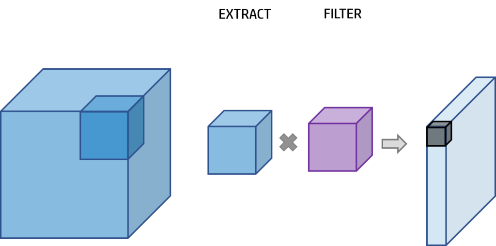
In the convolution operation, the input image will be the first blue square. We will get a little square that will be the same size of the filter (purple square) in width, height and depth and we will get a unique value (gray square). We will do this repeatedly to cover the entire input image.

The final depth of the output image of the convolution layer will be 1 but the witdh and the height will vary.

A convolutional layer will have some hyper-parameters:

• Input image size (I)
• Kernel size (K)
• Stride (S)
• Padding (P)

STRIDE (S)

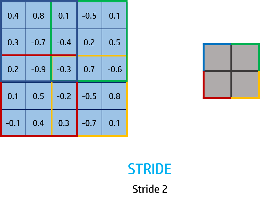
It’s an integer number that will be the number of steps we need to move to get an extract of the input image. When the extract has reached the latest position in the row it will go the stride number steps in the column movement.

In this example, the stride is 2 so we will move 2 steps each time. Each color represent a new extract of the input image. The size of this extract is 3x3x1 so the filter will have the same size.

PADDING (P)

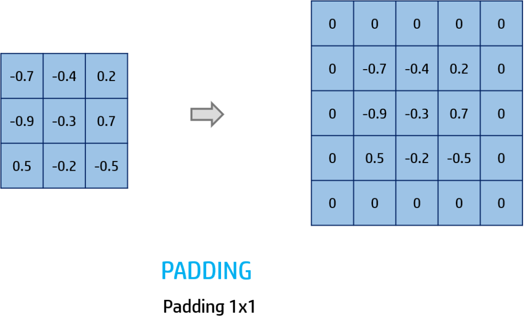
We will put a zero padding around the image. The padding integer number will be the size of it.

For example, if we have padding 1 we will put only one line of zeros around the image:

With all of this paramets we will be able to calculate the final output image size:

$$size=\frac{I+2P-K}{S}+1$$

For example if we have a padding of 1, stride 1 and an input image of 28x28x3 and the kernel 5x5x3, the output size when we apply the convolution operation of the image will be 24.

Now we will see a mathematical example of the convolution operation:

We will operate the convolution of $I*F$ and get the output green image with the convolutional operation formula.

Now we will move to the Activation Layer:

ACTIVATION LAYER

When we apply the convolution operation, we will normally use an activation layer to handle which values will be activated and which not.

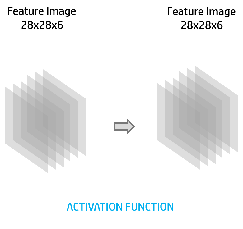
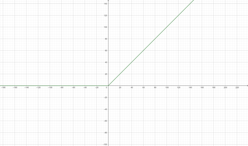
There are multiple activation functions but the most used for ConvNets is the ReLU function:

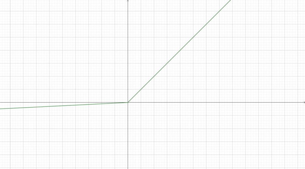
The RELU also has some variants such as PReLU:

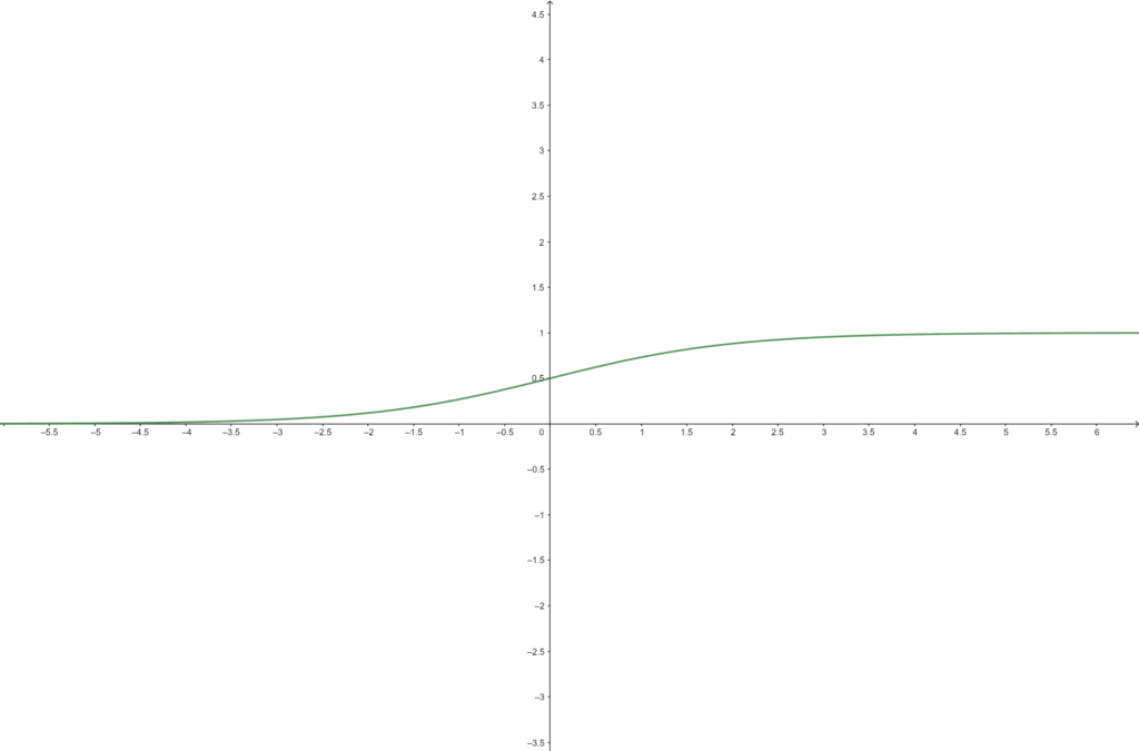
Also we can use the sigmoid function but this activation is usually used in other types of network such as the Feed-Forward Neural Network.

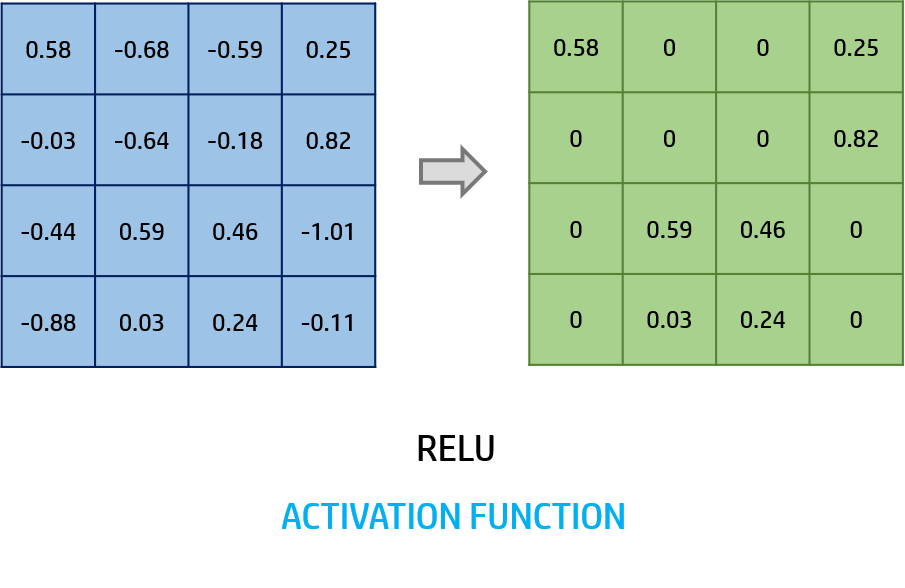
To calculate the output of the activation layer we will apply the activation function to each value and get a feature image of the same size as the input but with the values activated.

There is also a very important layer to simplify the image:

POOLING LAYER

This layer will usually be applied after the activation layer. It’s used to reduce the size in width and height of an image.

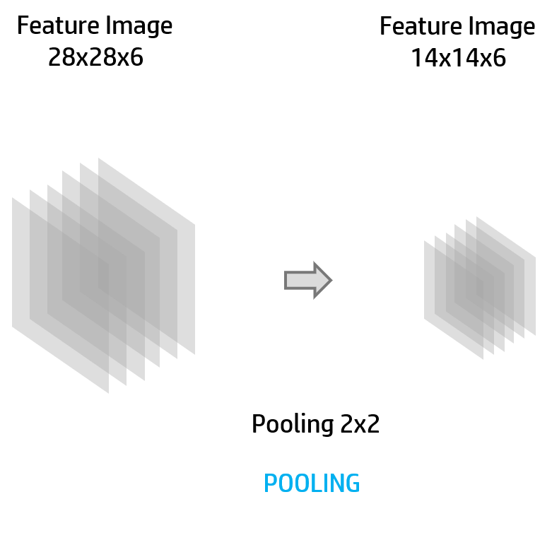
In this example the image have been reduced by the half of the original size.

In the pooling layer there are some hyper parameters:

• Size of pooling (similar to the size of the filter)

With the extract of the original image with the size of pooling we will apply the pooling)

• Stride (same as the convolutional stride)

The pooling can be done in two main methods:

• Max pooling

In the extract of the image we will only take the highest value and assigned it to the output image

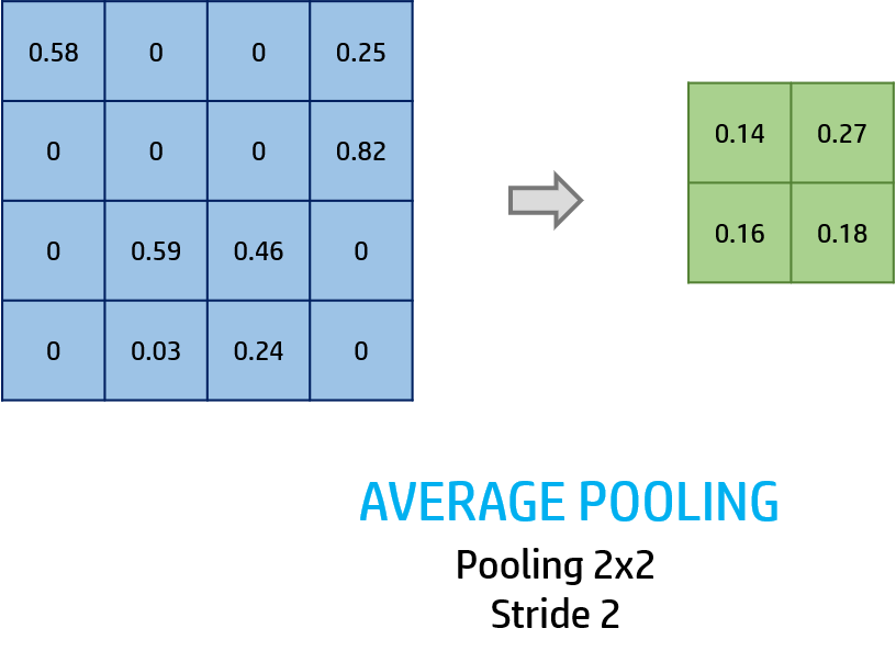
• Average pooling

However, with the average value, the ouput value will be the average of the extract of the image.

This is an example of the average pooling size of 2×2 with stride 2:

Now we will start with the other layers that are very similar to the feed-forward network.

FULLY CONNECTED LAYER

When we finally do all the previous layers we will finally get output final image and all the image will be reduced to an unidimensional array for the input array of the fully connected layer. This is also called flattening and we can apply a batch normalization. This will only be done in the first fully connected layer.

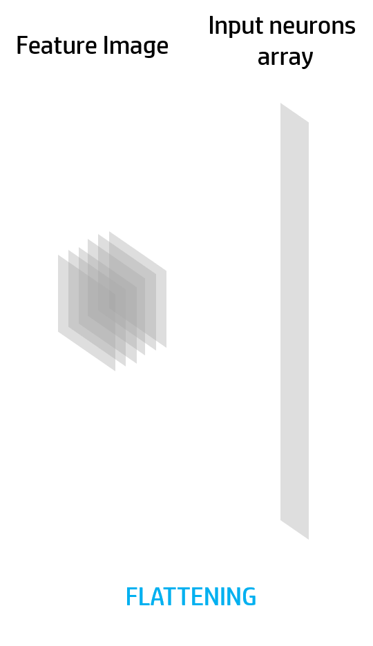
Each fully connected layer will be completely connected to the next layer. This layers will have some predifined neurons that will store a value.

Wen we want to update the network, in this layer we will do the feed-forward function.

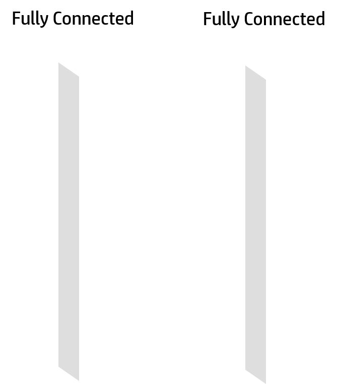
The feed-forward function in this layer is the same as the feed-forward explained in the Feed-Forward Neural Network tutorial. With the input that in this case will be the output of another layer and the weights that connected two fully connected layers we will calculate the next neurons values.

Also, as we will apply an activation function such as the ReLU, Sigmoid or Hiperbolic Tanh after the feed-forward.

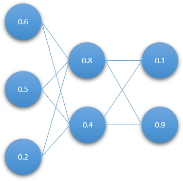
In the example you can see a traditional feed-forward neural network. If we are in a convolutional layer they will be fully connected layers, in this case 3 layers.

However the output layer will give the final prediction of the entire ConvNet and we will treat the data in a different way.

OUTPUT LAYER

This layer will be always the final layer of the network and will have a different activation function. This values will be the predictions of the neural network. If we are in image classification they will be the prediction confidence of the network.

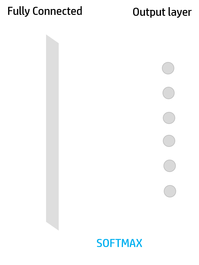
This layer will have an special activation function called Softmax that will depend on all the output of the final layer.

$$\sigma(a)_j=\frac{e^{a_j}}{\sum_{k}{e^{a_k}}}$$

Where $\sigma(a)$ is the activation function and $j$ is the actual neuron we want to activate. The sum will loop through all the output neuron values with position $k$.

CONVOLUTIONAL NEURAL NETWORK ARCHITECTURES

With all of this layers we will can combine these and create different architectures depending on their use we want to give them.

If we want to use it for digit or small RGB images we can use the Le-NET architecture (1998)

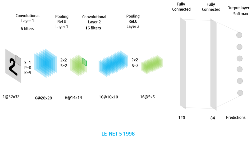
Firstly we have too iterations of the Convolution-ReLU-Pooling and the we flaten the final feature images and assign them to a Feed-Forward Neural Network of 2 hidden layers (fully connected layers). Finally we apply the softmax activation to the output layer.

We can use also this architecture for RGB images so the input image will have 3 channels:

There are many architecture that we can use for image classification. We have the Alex Net (2012), ResNet, DenseNet that are more modern architectures and are used nowadays. To understand deeply these convolutional neural networks I recommend you to see this link: https://www.jeremyjordan.me/convnet-architectures/.

In this presentation you will be able to see the images and the information you must know to understand neural networks.

[embeddoc url=”https://tutorials.retopall.com/wp-content/uploads/2019/02/Convolutional-Neural-Network-2.pptx” download=”all” viewer=”microsoft”]